Image classification with Vision Transformer
Author: Khalid Salama
Date created: 2021/01/18
Last modified: 2021/01/18
Description: Implementing the Vision Transformer (ViT) model for image classification.
Introduction
This example implements the Vision Transformer (ViT) model by Alexey Dosovitskiy et al. for image classification, and demonstrates it on the CIFAR-100 dataset. The ViT model applies the Transformer architecture with self-attention to sequences of image patches, without using convolution layers.
Setup
import os

os.environ["KERAS_BACKEND"] = "jax"  # @param ["tensorflow", "jax", "torch"]

import keras
from keras import layers
from keras import ops

import numpy as np
import matplotlib.pyplot as plt
Prepare the data
num_classes = 100
input_shape = (32, 32, 3)

(x_train, y_train), (x_test, y_test) = keras.datasets.cifar100.load_data()

print(f"x_train shape: {x_train.shape} - y_train shape: {y_train.shape}")
print(f"x_test shape: {x_test.shape} - y_test shape: {y_test.shape}")
x_train shape: (50000, 32, 32, 3) - y_train shape: (50000, 1)
x_test shape: (10000, 32, 32, 3) - y_test shape: (10000, 1)
Configure the hyperparameters
learning_rate = 0.001
weight_decay = 0.0001
batch_size = 256
num_epochs = 10  # For real training, use num_epochs=100. 10 is a test value
image_size = 72  # We'll resize input images to this size
patch_size = 6  # Size of the patches to be extract from the input images
num_patches = (image_size // patch_size) ** 2
projection_dim = 64
num_heads = 4
transformer_units = [
    projection_dim * 2,
    projection_dim,
]  # Size of the transformer layers
transformer_layers = 8
mlp_head_units = [
    2048,
    1024,
]  # Size of the dense layers of the final classifier
Use data augmentation
data_augmentation = keras.Sequential(
    [
        layers.Normalization(),
        layers.Resizing(image_size, image_size),
        layers.RandomFlip("horizontal"),
        layers.RandomRotation(factor=0.02),
        layers.RandomZoom(height_factor=0.2, width_factor=0.2),
    ],
    name="data_augmentation",
)
# Compute the mean and the variance of the training data for normalization.
data_augmentation.layers[0].adapt(x_train)
Implement multilayer perceptron (MLP)
def mlp(x, hidden_units, dropout_rate):
    for units in hidden_units:
        x = layers.Dense(units, activation=keras.activations.gelu)(x)
        x = layers.Dropout(dropout_rate)(x)
    return x
Implement patch creation as a layer
class Patches(layers.Layer):
    def __init__(self, patch_size):
        super().__init__()
        self.patch_size = patch_size

    def call(self, images):
        input_shape = ops.shape(images)
        batch_size = input_shape[0]
        height = input_shape[1]
        width = input_shape[2]
        channels = input_shape[3]
        num_patches_h = height // self.patch_size
        num_patches_w = width // self.patch_size
        patches = keras.ops.image.extract_patches(images, size=self.patch_size)
        patches = ops.reshape(
            patches,
            (
                batch_size,
                num_patches_h * num_patches_w,
                self.patch_size * self.patch_size * channels,
            ),
        )
        return patches

    def get_config(self):
        config = super().get_config()
        config.update({"patch_size": self.patch_size})
        return config
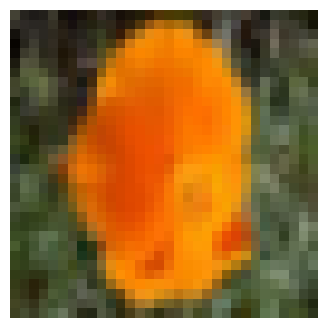
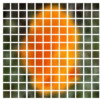
Let's display patches for a sample image
plt.figure(figsize=(4, 4))
image = x_train[np.random.choice(range(x_train.shape[0]))]
plt.imshow(image.astype("uint8"))
plt.axis("off")

resized_image = ops.image.resize(
    ops.convert_to_tensor([image]), size=(image_size, image_size)
)
patches = Patches(patch_size)(resized_image)
print(f"Image size: {image_size} X {image_size}")
print(f"Patch size: {patch_size} X {patch_size}")
print(f"Patches per image: {patches.shape[1]}")
print(f"Elements per patch: {patches.shape[-1]}")

n = int(np.sqrt(patches.shape[1]))
plt.figure(figsize=(4, 4))
for i, patch in enumerate(patches[0]):
    ax = plt.subplot(n, n, i + 1)
    patch_img = ops.reshape(patch, (patch_size, patch_size, 3))
    plt.imshow(ops.convert_to_numpy(patch_img).astype("uint8"))
    plt.axis("off")
Image size: 72 X 72
Patch size: 6 X 6
Patches per image: 144
Elements per patch: 108


Implement the patch encoding layer
The PatchEncoder layer will linearly transform a patch by projecting it into a
vector of size projection_dim. In addition, it adds a learnable position
embedding to the projected vector.
class PatchEncoder(layers.Layer):
    def __init__(self, num_patches, projection_dim):
        super().__init__()
        self.num_patches = num_patches
        self.projection = layers.Dense(units=projection_dim)
        self.position_embedding = layers.Embedding(
            input_dim=num_patches, output_dim=projection_dim
        )

    def call(self, patch):
        positions = ops.expand_dims(
            ops.arange(start=0, stop=self.num_patches, step=1), axis=0
        )
        projected_patches = self.projection(patch)
        encoded = projected_patches + self.position_embedding(positions)
        return encoded

    def get_config(self):
        config = super().get_config()
        config.update({"num_patches": self.num_patches})
        return config
Build the ViT model
The ViT model consists of multiple Transformer blocks,
which use the layers.MultiHeadAttention layer as a self-attention mechanism
applied to the sequence of patches. The Transformer blocks produce a
[batch_size, num_patches, projection_dim] tensor, which is processed via an
classifier head with softmax to produce the final class probabilities output.
Unlike the technique described in the paper,
which prepends a learnable embedding to the sequence of encoded patches to serve
as the image representation, all the outputs of the final Transformer block are
reshaped with layers.Flatten() and used as the image
representation input to the classifier head.
Note that the layers.GlobalAveragePooling1D layer
could also be used instead to aggregate the outputs of the Transformer block,
especially when the number of patches and the projection dimensions are large.
def create_vit_classifier():
    inputs = keras.Input(shape=input_shape)
    # Augment data.
    augmented = data_augmentation(inputs)
    # Create patches.
    patches = Patches(patch_size)(augmented)
    # Encode patches.
    encoded_patches = PatchEncoder(num_patches, projection_dim)(patches)

    # Create multiple layers of the Transformer block.
    for _ in range(transformer_layers):
        # Layer normalization 1.
        x1 = layers.LayerNormalization(epsilon=1e-6)(encoded_patches)
        # Create a multi-head attention layer.
        attention_output = layers.MultiHeadAttention(
            num_heads=num_heads, key_dim=projection_dim, dropout=0.1
        )(x1, x1)
        # Skip connection 1.
        x2 = layers.Add()([attention_output, encoded_patches])
        # Layer normalization 2.
        x3 = layers.LayerNormalization(epsilon=1e-6)(x2)
        # MLP.
        x3 = mlp(x3, hidden_units=transformer_units, dropout_rate=0.1)
        # Skip connection 2.
        encoded_patches = layers.Add()([x3, x2])

    # Create a [batch_size, projection_dim] tensor.
    representation = layers.LayerNormalization(epsilon=1e-6)(encoded_patches)
    representation = layers.Flatten()(representation)
    representation = layers.Dropout(0.5)(representation)
    # Add MLP.
    features = mlp(representation, hidden_units=mlp_head_units, dropout_rate=0.5)
    # Classify outputs.
    logits = layers.Dense(num_classes)(features)
    # Create the Keras model.
    model = keras.Model(inputs=inputs, outputs=logits)
    return model
Compile, train, and evaluate the mode
def run_experiment(model):
    optimizer = keras.optimizers.AdamW(
        learning_rate=learning_rate, weight_decay=weight_decay
    )

    model.compile(
        optimizer=optimizer,
        loss=keras.losses.SparseCategoricalCrossentropy(from_logits=True),
        metrics=[
            keras.metrics.SparseCategoricalAccuracy(name="accuracy"),
            keras.metrics.SparseTopKCategoricalAccuracy(5, name="top-5-accuracy"),
        ],
    )

    checkpoint_filepath = "/tmp/checkpoint.weights.h5"
    checkpoint_callback = keras.callbacks.ModelCheckpoint(
        checkpoint_filepath,
        monitor="val_accuracy",
        save_best_only=True,
        save_weights_only=True,
    )

    history = model.fit(
        x=x_train,
        y=y_train,
        batch_size=batch_size,
        epochs=num_epochs,
        validation_split=0.1,
        callbacks=[checkpoint_callback],
    )

    model.load_weights(checkpoint_filepath)
    _, accuracy, top_5_accuracy = model.evaluate(x_test, y_test)
    print(f"Test accuracy: {round(accuracy * 100, 2)}%")
    print(f"Test top 5 accuracy: {round(top_5_accuracy * 100, 2)}%")

    return history


vit_classifier = create_vit_classifier()
history = run_experiment(vit_classifier)


def plot_history(item):
    plt.plot(history.history[item], label=item)
    plt.plot(history.history["val_" + item], label="val_" + item)
    plt.xlabel("Epochs")
    plt.ylabel(item)
    plt.title("Train and Validation {} Over Epochs".format(item), fontsize=14)
    plt.legend()
    plt.grid()
    plt.show()


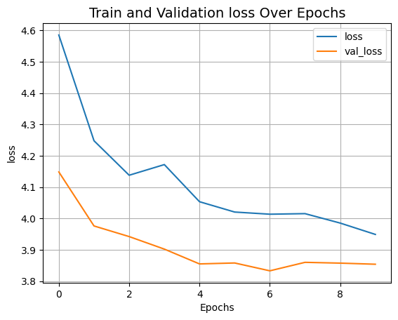
plot_history("loss")
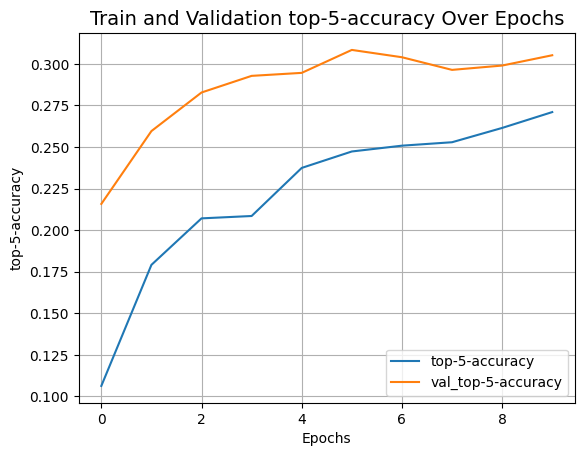
plot_history("top-5-accuracy")
Epoch 1/10
...
Epoch 10/10
 176/176 ━━━━━━━━━━━━━━━━━━━━ 449s 3s/step - accuracy: 0.0790 - loss: 3.9468 - top-5-accuracy: 0.2711 - val_accuracy: 0.0986 - val_loss: 3.8537 - val_top-5-accuracy: 0.3052

 313/313 ━━━━━━━━━━━━━━━━━━━━ 66s 198ms/step - accuracy: 0.1001 - loss: 3.8428 - top-5-accuracy: 0.3107
Test accuracy: 10.61%
Test top 5 accuracy: 31.51%


After 100 epochs, the ViT model achieves around 55% accuracy and 82% top-5 accuracy on the test data. These are not competitive results on the CIFAR-100 dataset, as a ResNet50V2 trained from scratch on the same data can achieve 67% accuracy.
Note that the state of the art results reported in the paper are achieved by pre-training the ViT model using the JFT-300M dataset, then fine-tuning it on the target dataset. To improve the model quality without pre-training, you can try to train the model for more epochs, use a larger number of Transformer layers, resize the input images, change the patch size, or increase the projection dimensions. Besides, as mentioned in the paper, the quality of the model is affected not only by architecture choices, but also by parameters such as the learning rate schedule, optimizer, weight decay, etc. In practice, it's recommended to fine-tune a ViT model that was pre-trained using a large, high-resolution dataset.